月份: 六月 2016

Bioc2016第三天的會議也相當精彩，早上的科學新知演講開場由Rob Tibshirani史丹佛著名統計學家，他的研究成果非常豐富，從早年的bootstrap到近年來不斷思考一些statistic inference selection的方法學。

有史丹佛教授William Greenleaf 講解他在分析ATAC-seq資料的過程和背後的思維，ATAC-seq簡單來說就是用定序的技術來“間接”探討chromatin的結構，也就是epigenetics的領域，Greenleaf的背景非常數理，是應用物理學、化學出身，講話給人一種加強版的福爾摩斯，剛好其就是英國人。

史丹佛教授Stephen Montgomery則是早期做GWIS的研究、慢慢開始有eQTL和做allele specific及gene variation間的分析。

系列一

Bioconductor第二天開始的會議，就變成白天已scientific talk為主，而下午則是workshop的方式，scientific talk又會分成科學演講（主要由教授來分享）和社群的演講（偏向目前新開發之package使用分享）。

一開始由柏克萊大學Sandrine Dudoit生物統計教授分享主題為Identification of Novel Cell Types in the Brain using Single-Cell Transcriptome sequencing，其本身研究發展許多可用來標準化RNAseq的方法。

再來則是史丹佛大學的Susan Holmes(其個人網站有許多之前talk的資料)分享題目為Muticomponent data inegration for the Human Microbiome，其本身研究使用無母數的分析像是SVD、bootstrap、MCMC來探討生物現象所產出的資料，最近也有研究如愛滋病病患使用藥物後其microbiome的改變。

Jenny Bryan（他個人頁面有許多學習資源鏈結）教授則是分享其開發的googlespreadsheet package 其串連goolge doc API去讓使用者可以輕鬆地將google spreadsheet輸入到R中來做進一步的處理。Michael Love給了一個有Bioconductor Workflows Following Fast, Lightweight RNA Transcript Quantifiers的talk，他本身與哈佛生統教授Rafael Irizareay在edx開了一系列biostatistic的課。發展slidify的Ramnath Vaidya則在講新的Html widget。

下午的workshop則教了許多其他的packages像是UC riverside的教授Thomas Girke來發表其所撰寫的systemPipeR，是一款可以直接在R中使用的pipeline工具（雖然部分功能有待加強），而華盛頓大學的James MacDonald則很仔細地探討各種目前常用R database其中qeury等細節的論輪（expressionSet,TxDb,OrgDb…..）

Bioconductor 算是R語言中對於生物資訊最重要的一個project，目前演進成一個龐大的社群，裡面眾多的協力者發展出很多High-throughput genomic data analysis的工具。

 

開始摸索mongoDB的第一件事情:安裝

$brew install mongodb


$mkdir -p /data/db


• 將所有的node之間的關係用一個巨大matrix來記錄，row代表是starting node，column代表是receiving node，但當這個network很巨大的時候，此種形式大部分的cell都會是空值。但資料小時候很一目了然。
  
  

• 直接用一個table記錄每個paired的關係，第一個column代表是starting node，第二個column則是receiving node，這種方式比較直覺，在資料量大的時候處理速度也會比sociomatrix建立的網絡還快，因為少去了很多empty data。
  
  

<

div>

#load the library
library(statnet)


#Creat a network object with sociometrix data format
netmat1 <- rbind(c(0,1,1,0,0),
                 c(0,0,1,1,0),
                 c(0,1,0,0,0),
                 c(0,0,0,0,0),
                 c(0,0,1,0,0))
rownames(netmat1) <- c("A","B","C","D","E")
colnames(netmat1) <- c("A","B","C","D","E")
net1 <- network(netmat1,matrix.type="adjacency")
class(net1)
summary(net1)
##Visualization
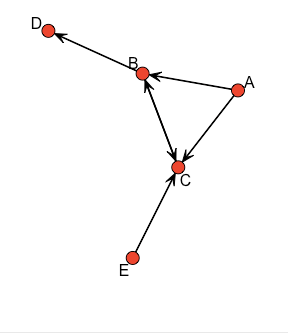
gplot(net1)
gplot(net1, vertex.col = 5, displaylabels =TRUE)
#Creat network object with edge list format
netmat2 <- rbind(c(1,2),
                 c(1,3),
                 c(2,3),
                 c(2,4),
                 c(3,2),
                 c(5,3))
net2    <- network(netmat2, matrix.type="edgelist")
network.vertex.names(net2) <- c("A","B","C","D","E")
summary(net2)


#Transform between the differnet data structure
as.sociomatrix(net1)
class(as.sociomatrix(net1))

all(as.matrix(net1) == as.sociomatrix(net1))
as.matrix(net1,matrix.type = "edgelist")

#-Managing Node and Tie attributes

#Node attribute
set.vertex.attribute(net1, "gender", c("F","F","M","F","M"))
net1 %v% "alldeg" <- degree(net1)
list.vertex.attributes(net1)
summary(net1)

get.vertex.attribute(net1,"gender")
net1 %v% "alldeg"

#Tie attribute
list.edge.attributes(net1)
set.edge.attribute(net1,"rndval",
                   runif(network.size(net1),0,1))
list.edge.attributes(net1)
summary(net1 %e% "rndval")
summary(get.edge.attribute(net1,"rndval"))

#example for the value netwrok and modify the edge attribute
netval1 <- rbind(c(0,2,3,0,0),
                 c(0,0,3,1,0),
                 c(0,1,0,0,0),
                 c(0,0,0,0,0),
                 c(0,0,2,0,0))
netval1 <- network(netval1,matrix.type="adjacency",ignore.eval=FALSE, names.eval="like") #use the vertex's vaule added to attribute
list.edge.attributes(netval1)
get.edge.attribute(netval1,"like")

as.sociomatrix(netval1)
as.sociomatrix(netval1,"like")

#--------------------------------------------------------------------
#igraph

#detach the statnet during the duplicate of function name
install.packages("igraph")
detach(package:statnet)
library(igraph)
#create from sociomatrix
inet1  <- graph.adjacency(netmat1)
class(inet1)
summary(inet1)
str(inet1)
#create from edge list
inet2 <- graph.edgelist(netmat2)
summary(inet2)


#modify the attribute
V(inet2)$name <- c("A","B","C","D","E")
E(inet2)$val  <- c(1:6)
summary(inet2)
str(inet2)


#--------------------------------------------------------------------
#Going back and forth between statnet and igraph
install.packages("intergraph")
library(intergraph)
class(net1)
net1igraph <- asIgraph(net1)
class(net1igraph)
str(net1igraph)


#Imporintg Netwrok data
detach("package:igraph",unload=TRUE)
library(statnet)
netmat3 <- rbind(c("A","B"),
                 c("A","C"),
                 c("B","C"),
                 c("B","D"),
                 c("C","B"),
                 c("E","C"))

net.df  <- data.frame(netmat3)
net.df
write.csv(net.df, file = "MyData.csv",
          row.names = FALSE)
net.edge <- read.csv(file = "MyData.csv")
net_import <- network(net.edge,matrix.type = "edgelist")
summary(net_import)

gden(net_import)

#Common Network Data Task

#Filtering Networks Based on Vertex or Edge Attribute Values
n1F <- get.inducedSubgraph(net1,
                           which(net1 %v% "gender" == "F"))

n1F[,]
gplot(n1F,displaylabels = TRUE)

deg <- net1%v% "alldeg"
n2  <- net1 %s% which(deg >1)
gplot(n2,displaylabels = TRUE)

#Removing Isolates
library(UserNetR)
data("ICTS_G10")
gden(ICTS_G10)
length(isolates(ICTS_G10))

n3 <- ICTS_G10
delete.vertices(n3,isolates(n3))
gden(n3)
length(isolates(n3))

#Filtering Based on Edge Values
data(DHHS)
d <- DHHS
gden(d)

op <- par(mar = rep(0,4))
gplot(d,gmode="graph",edge.lwd = d %e% 'collab',
      edge.col = "grey50", vertex.col = "lightblue",
      vertex.cex = 1.0, vertex.sides=20)

as.sociomatrix(d)[ 1:6,1:6]
list.edge.attributes(d)
as.sociomatrix(d,attrname="collab")[1:6,1:6]

table(d %e% "collab")

d.val <- as.sociomatrix(d,attrname="collab")
d.val[d.val < 3] <0
d.filt <- as.network(d.val, directed=FALSE,matrix.type="a",
                     ignore.eval=FALSE,names.eval="collab")
summary(d.filt, print.adj=FALSE)
gden(d.filt)
#Method to drawing
op <- par(mar = rep(0,4))
gplot(d.filt,gmode="graph",displaylabels = TRUE,vertex.col="lightblue",vertex.cex=1.3,
      label.cex=0.4, label.pos=5,
      displayisolates = FALSE)

#Advanced 
op <- par(mar = rep(0,4))
d.value <- as.sociomatrix(d,attrnment="collab")
gplot(d.filt,gmode="graph",thresh=2,vertex.col ="lightblue",vertex.cex=1.3,
      label.cex=0.4, label.pos=5,
      displayisolates = FALSE)
par(op)



#Transformating a directed network to non-directed network
net1mat <- symmetrize(net1, rule = "weak")
net1symm <- network(net1mat,matrix.type="adjacency")
network.vertex.names(net1symm) <- c("A","B","C","D","E")
summary(net1symm)

使用R做Network Analysis系列二

這一系列的學習是為了之後分析複雜生物網絡所準備，也是系統生物學中很重要的研究技巧，如何做network analysis，這邊用R 來做操作。

正常的descriptive statistic也會有所謂的5-number summary來描述一組資料的基本特性(最大值、最小值、中位數、25th位數、75th位數)。

同樣的道理，當我們面對一個網路，要如何了解他的基本性質也有五大特性可以來看

• Size：
  簡單來說就是一個network裡頭的節點（可稱作nodes, vertices或是actors），這個是基本上可以讓我們知道一個網絡的大小規模。
• Density：
  這邊的“密度”是指這網絡中點和點間聯繫數量相對於總數兩兩都連接的比值，也就是說假如有k個點，則當每個點都相互連接，則有k(k-1)的聯繫，在雙向的聯繫網絡中則算是有k(k-1)/2個聯繫，這就是網絡內點與點最大值，而實際上所有點相互間聯繫/點與點都聯繫的值就是這邊的density。
• Components：
  這邊是指一個網絡中有幾個group，這邊的group裡的點都沒有跟彼此相互聯繫。
• Diameter：
  這邊看的是這網路中距離最遠的兩個點，其之間經過的節點數
• Clustering Coefficient
  這項指標就比較難理解一點，這邊看的是網絡裡面的點以特定節點為中心聚合的比例，以三個點互相連結為最小單位，簡單說就是當兩個點都有共同連接點時，這兩個點也相互連接的傾象。

首先必須先安裝statnet和UserNetR兩個packages，其中UserNetR是這本User’s guide to network analysis in R 裡所有示範資料的packages，而statnet則是做network analysis的package。

library(UserNetR)
library(statnet)
data(Moreno)

先簡單把Moreno這組資料畫圖

gender <- Moreno %v% "gender"
plot(Moreno, vertex.col = gender + 2, vertex.cex = 1.2)

用 network.size函數來看這個network object裡面的節點數

#5-number summary
 #1st: Size
network.size(Moreno)

用gden函數他會算出這network裡頭的density，一個介於0到1的數值，即目前這個網絡中所有連結數量與最大連結數量的比值

 #2nd: Density, range from 0 to 1, unidirect or direct
gden(Moreno)

直接算是這個網絡中幾個無互相聯繫的subgroup

 #3rd: Components, subgroups
components(Moreno)

算出網絡中兩者連結需要經過的最大節點數，並且可以算出整個網絡的cluster coefficient

 #4th: Diameter, how compact the network are
lgc <- component.largest(Moreno,result="graph")
gd  <- geodist(lgc)
max(gd$gdist)

 #5th: Cluster Coefficient, range from 0 to 1 ,measure the transitivity
gtrans(Moreno,mode="graph")

參考資料：Luke, Douglas A. A User’s Guide to Network Analysis in R

分享在使用dplyr時遇到的狀況：

這是一個很平常的將檔案讀進來的步驟，但比較特別的是我使用了readr package的read_csv來讀取。

而讀進來後的nor.count長這樣

接下來我做這些事情，將column重新命名，且把gene list的名字提取出來，為了等會轉換成單純的matrix，提取後在使用dplyr的select，可以直接去掉gene的這行。當nor.count為完全的numeric matrix時，我將數值做log2 transformatiopn，接下來便要開始來處理資料

接者想要把資料裡的row不等於0濾掉，所以使用filter上面 （錯誤訊息發生）

從錯誤訊息，看起來可能是nor.count的格式不符合，再來看一下現在nor.count變成什麼樣子了

這時候發現一個奇怪的地方，在nor.count的structure中，看到gene下面還有一個data.frame Gene!!

原來是在tbl_df的object中，用傳統的方式subset他還是會保持tbl_df，不會因此變成atomic vector的形式

像上面這種是很常見的subsetting的方法，subset完後，就照下面的方式再塞回data.frame中，但在tbl_df的object用此操作則會發生問題，這樣就會變成在data.frame裡面塞入一個data.frame，而這種形式就會造成之後的function無法處理

所以面對tbl_df就必須乖乖的使用

把gene.list給放回去！